Logistic Regression from scratch

Logistic Regression is one the more simpler classification model that is heavily used for inference focused data analysis tasks. In this post I will be explaining the basic theory as well as implementing the standard Logistic Regression from scratch.

Before we begin, a quick introduction to Logistic Regression. It is a regression model where the dependent variable is categorical in nature. The standard Logistic Regression deals with only binary data i.e. the dependent variable can take only one of two possible values for e.g. it can be either 1 or 0. The way Logistic Regression changes a value returned by a regression equation i.e. a line equation to a probability value for one of the 2 classes is by squishing the regression value between 0 and 1 using the sigmoid function which is given by $$ f(x) = \frac{1}{1 + e^{-X}} $$ Above X represents the output of the regression equation and hence can also be replaced by the actual linear equation \( w^Tx \). Given the nature of the exponential function f(x) will reach 1 and 0 at x = \(\infty, - \infty\) respectively. The aim of learning a Logistic Regression function is figuring out the weight vector w. This is what we are going to do next, but before that a small note as in any regression equation we should a \(w_0\) bias term in the equation as well, going forward in all the equations we assume that the \(w_0\) is added to \(w^Tx\) by adding an additional dimension with value 1 to x.

So a way to figure out the weight vector w is to essentially find weights that maximizes the likelihood of observing the given sample. This method is know as MLE Maximum Likelihood Estimation. Lets figure out what this function that we want to maximize will look like. As Logistic regression is a binary classification so the probability distribution can be modelled using Bernoulli Distribution. $$ P(y | x) = f(x)^y(1-f(x))^{1-y} $$ Remember that our objective here is to maximize the likelihood of observing the given samples, another way of saying this is that we want to maximize the correct class probability of each of the samples. This can be written as: $$ l(w) = \sum_{l=1}^N P(y_l | x_l, w) $$ l(w) is the function that we want to maximize but we don't have a closed form solution of it we can't really get the optimal weight values directly. Instead what we will use Gradient Ascent (just performing the reverse of gradient descent as we have to maximize the function not minimize it) to figure it out. Even though we can use Gradient Ascent on the function above directly, solving such equation after taking their log makes things a lot easier mathematically. $$ ln(l(w)) = \sum_{l=1}^N ln(P(y_l | x_l, w)) \\ = \sum_{l=1}^N yln(\frac{1}{1 + e^{-w^Tx}}) + (1-y)ln(1 - \frac{1}{1 + e^{-w^Tx}}) \\ = \sum_{l=1}^N yln(\frac{1}{1 + e^{-w^Tx}}) + (1-y)ln(\frac{e^{-w^Tx}}{1 + e^{-w^Tx}}) \\ = \sum_{l=1}^N ln(\frac{e^{-w^Tx}}{1+ e^{-w^Tx}}) - yln(e^{-w^Tx}) \\ = \sum_{l=1}^N (y - 1)w^Tx - ln(1+ e^{-w^Tx}) \\ $$ Now that the equation is simplified a bit lets take its derivative w.r.t. to the variable we want to maximize the function's value which is w. As w is multi-dimensional we would be taking the derivative with respect to only of the dimension at one time $$ \frac{\partial l(w)}{\partial w_i} = \sum_{l=1}^N (y^l - 1)x^l_i + \frac{1}{1+ e^{-w^Tx^l}}*e^{-w^Tx^l}x^l_i \\ = \sum_{l=1}^N x_i((y^l - 1) + \frac{1}{1+ e^{-w^Tx^l}}*e^{-w^Tx^l}) \\ = \sum_{l=1}^N x_i(y^l + \frac{e^{-w^Tx^l} - 1 - e^{-w^Tx^l}}{1+ e^{-w^Tx^l}}) \\ = \sum_{l=1}^N x_i(y^l - \frac{1}{1+ e^{-w^Tx^l}}) \\ = \sum_{l=1}^N x_i^l(y^l - P(y^l | x^l_i, w)) $$ P.S. l(w) above is same as ln(l(w)) I just changed the notation a bit to make the equation look a bit simpler The update equation would look like $$ w_{i+1} = w_i + n\sum_{l=1}^N x_i^l(y^l - P(y^l | x^l, w)) $$ Here n represents the learning rate Now that we have the equations worked out lets build it out

def sigmoid(x):
    return 1.0/(1 + np.exp(-x))

def update_w(x, y, w, learningRate):
    #This function performs one round of weight update using all the samples
    scores = np.dot(x, w) #calculation wTx
    predictionVals = sigmoid(scores) #getting the probabilities
    predictionError = y - predictionVals # yl−P(yl|xl,w)
    gradient = np.dot(x.T, predictionError) #This operation calculates the gradient for all dimension at once
    updateVal = learningRate * gradient
    return w + updateVal

def logistic_regression(x, y, learningRate, iterations=30000, add_intercept=True):
    if add_intercept:
        intercept = np.ones((x.shape[0], 1))
        x = np.hstack((x, intercept))
    # initializing w to be all zeroes
    w = np.zeros(x.shape[1])
    for it in xrange(iterations):
        w_new = update_w(x, y, w, learningRate)
        w = w_new
    return w

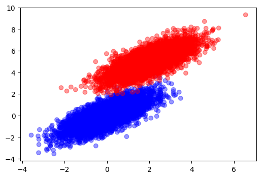
Thats it. Above is all the code required to make Logistic Regression work. Now to test it we will need a dataset. Lets Generate one.

numSamples = 5000
negativeSamples = np.random.multivariate_normal([0, 0], [[1, .75],[.75, 1]], numSamples)
positiveSamples = np.random.multivariate_normal([2, 5], [[1, .75],[.75, 1]], numSamples)
samples = np.concatenate((negativeSamples, positiveSamples))
labels = np.concatenate((np.zeros(numSamples), np.ones(numSamples)))
plt.scatter(samples[:, 0], samples[:, 1], c = map(lambda x: 'b' if x == 0 else 'r', labels), alpha = 0.4)

from sklearn.linear_model import LogisticRegression
weights = logistic_regression(samples, labels, 1e-4, 30000, True)
mdl = LogisticRegression(C=1e15, max_iter =30000)
mdl.fit(samples, labels)
print mdl.coef_, mdl.intercept_
print weights

[[-3.7105873  7.9527151]] [-16.16972923]
[ -3.39479514   7.28384609 -14.78495992]

I set C to a very high value so as to discard regularization as I haven't added a term for regularization in my implementation. The weights obtained are very close which should be the case if the implemented algorithm is correct. Though the weights are close, sklearn's implementation is way faster. This is because sklearn uses a highly optimized solver.

In closing I would like to add that, even though our weights were quite close to the ones obtained by sklearn, it never makes sense to implement such systems from scratch to run on production systems.