Music Genre Classification Using Convolutional Neural Network

This post provides a simple and brief overview of what Covolutional Neural Networks are and how to use them to predict the genre of any songs. I will go into a lot of details so buckle up cause this is gonna be a long post

Convolutional Neural Network

Convolutional Neural Networks (CNNs) are a special type of Neural Network which have special convolutional layers in addition of the usual fully connected layers. These convolutional layers are notthing but filters which slide over the data to produce output. The history of CNNs can be traced to Image processing and recognition. Basically, earlier for any sort of image recognition what people used to do was to generate hand crafted features based on their intuition and understanding of the problem domain. Take for example the following task of recognizing the digit in an image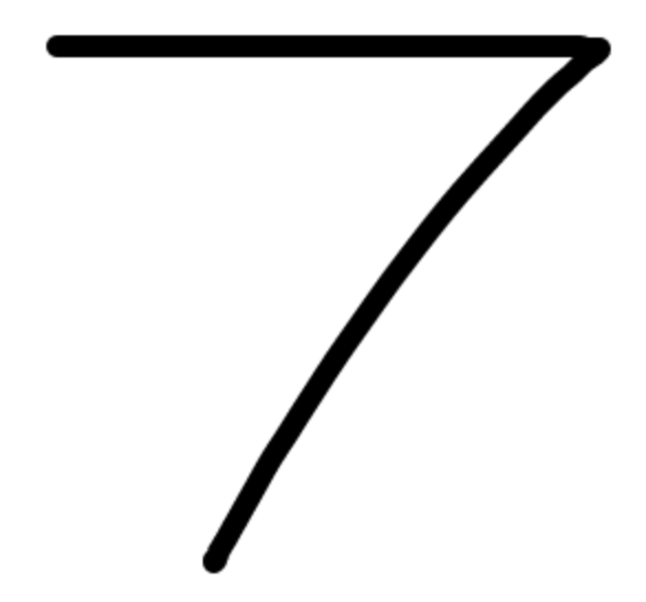

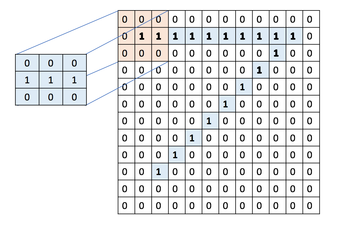
Here, a simple approach would be to maybe look for edges in the images and go from there. To capture these edge what is normally applied is a filter that would slide through the image, perform a dot product with the image values and record if it observes any edge in it or not. Something like the following would happen if we want to slide an edge filter over the image of 7.

A Convolutional Neural Network does exactly this. It has a bunch of such filters which it slides over images to generate what are called activation map which is nothing but the dot product of the filter and a small part of the image (Note: the depth of the filter is same as that of the image so if the image has 3 channels Red Green and Blue, then the depth of the filter will be automatically set to 3). The awesome thing about a convolutional network though is that you don't have to worry about designing the filters themselves. The training portion of the network takes care of that. And this is the exact thing that made CNNs so popular as before the major challenge in any image recognition task was to come with the hand crafted features and corresponding filters for them.

So in essence CNNs are neural networks with an additional set of learnable filters which are used to identify features in the dataset. The typical architecture of any convolutional neural network looks something like this:

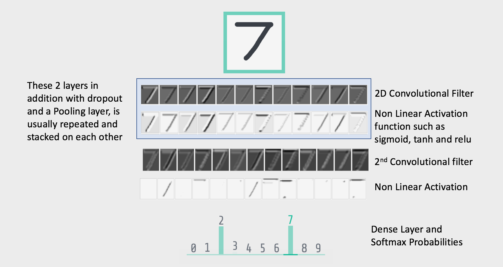
So I missed a few key terms such as Non linear Activation, Pooling and dropout. Lets now understand briefly what these terms are:

Non Linear Activation

Non Linear Activation functions are what gives neural networks their advantage over other machine learning methods. These activations are inspired from the process that happen in our own neuron. However, they are really just a very crude and rudimentary approximation of the actual process. Common Activation functions are: sigmoid, tanh and relu. Though sigmoid in the most known function in all of them but sadly it is also the least used one. The most commonly used activation function is relu, which is simply Max(0, x) where x is the input to the activation function. The reason relu works better than other activation functions is that it does not saturate, where as both sigmoid and tanh saturate as they reach their min or max value which causes the gradients to become very very small causing the network to not learn.

Pooling

Pooling is a way to reduce the size of the input to any of the layers in the network. Basically as done with the filters before a matrix is slided over the output of the Non Linear Activation layer. This matrix however is not learnable and has to be specified while describing the network. There are many type of pooling operations such as min, max, average, etc. . The most common type of pooling is max pooling, in it a window of size specified during network construction. This window is slid over the input to the layer and the max value is found to replace the window with that max value.

Dropout

Dropout is a hyperparameter that specifies how many of the neurons should be deactivated at each training step. A simple hand wavy explaination of why would anyone want to deactivate any neurons during training is that it sort of creates an ensembles of networks, someting similar to what happens in a Random Forest or any other Boosted tree methods. Basically, by deactivating some random neurons you ensure that the models does not learn only in a particular direction but rather tries and generalize as much as possible. This is also the reason why Dropout is used as a regularization method to improve model generalization. Another reason why people use dropout is that by randomly deactivating certain neurons, you can force gradients to flow through the network making it learn better.

Uptil now we only covered what the typical convolutional neural network looks like, we have not discussed how a model learns all the things it has to learn. This process is the same as any regular neural network and is known as Back Propogation. To describe what Back Propagation is and how is everything calculated will take a post of its own. But to just describe it briefly it is a way by which based on the output of the last layer and its comparison with the actual class labels, the weights of the layers are updated one by one. It goes one layer at a time starting from the last, then the second last and so on till the first layer. This is why the method is called Back Propogation as the updates the propogated from the last to the first layer.

If you are interested in understanding the maths behind all the topics I covered above I would highly recommend that you go through Stanford's cs231n taught by Andrej Karpathy. It is a good course but if you don't have time and just want to understand the concepts discussed here you can go through the following as well here , here and here. If you want to see how the output of various layers in a convolutional layer looks like visit here , it is a real fun example that helps in understanding a CNN

Music Genre Prediction

Now that we have briefly discussed what a CNN is and how it functions. Lets now see how it can be applied to predict the genre of a song. But first lets go through how we are going to represent a song and how this CNN will be different to the ones we discussed till now. Finally before I start I am using GTZAN dataset for training my neural network

Feature Engineering - Mel Spectogram

The normal sampling rate of any audio sample is generaly 44100 Hz i.e. 44,100 samples are taken per second. If we were to give raw audio clip like to we do for images and even if the clips are of size 100ms (this is what we will do a bit later), the input layer would need 4410 neurons. This is not particularly a lot but if you want to train it on your local machine, this might cause an issue as the for each neuron in the network we have to store some data for back propogation and training. So if there are a lot of neurons in the network, more than for which the data could be stored in the RAM, the training time will be very very high.

So in order to represent the audio file we will use something that is known as a Mel Spectogram. It is basically a spectogram with values mapped down to Mel scale i.e. log scale. Mel Spectogram represents the frequency distribution over time. The reason why I am using this and not anything else is that I found Mel Spectogram to be used in a lot of audio processing tasks. Lets now see how these Mel Spectogram look for two very different genres Blues and Jazz

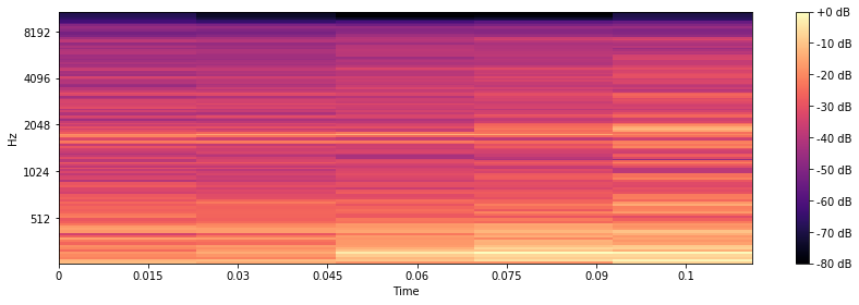
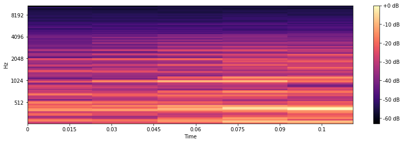
As we can observe from the two spectograms there is obviously a difference between the two spectogram, which should be the case as the two genre are quite different.

Input Preperation

All the audio files in the GZTAN dataset are 30 seconds in length. One way would be to create spectogram on whole audio file. However, as the GZTAN dataset contains only 1000 songs, that won't be enough to train the network. So, instead what I did was to take 100 ms windows over the audio files and compute the Mel Spectogram for each of these little windows for each of the file. The Mel Spectrogram calculation was performed using python's Librosa library, the number of FFT components was set to 128. The Mel Spectrogram for each 100 ms second window is represented by a vector of shape (128, 5). To ensure consistency I limited the window calculation to 599, i.e. for each audio I calculated Mel Spectogram for only 599 windows. This was the most time consuming phase of this experiment because even with an 3.4 Ghz Quad core i7, processing each file took approximately 120 seconds.

Network Architecture

As we computed 599 windows over each of the file our dataset now has a shape of (1000, 599, 128, 5). If we take each of the window as a sample then we have 599000 samples, which is more than enough to train a simple network. Before we proceed there is one more thing that I should clarify, even though the spectogram looks like an image we are not going to use 2D convolutional filter. We instead are going to use 1D convolutional filters, which would slide along the time dimension and not the frequency Dimension (I decided on using time as the dimension of convolution as that is what I found other folks to be doing as well). To make sure out filters move accross the time dimension and not the frequency dimension we need to pivot each of our (128, 5) sample. One can use Numpy's transpose function for this task. So finally, our dataset is ready and it looks like (599000, 5, 128). All that is left now is to build our model, split the data set into train, validation and test and train out model. For building the model I will be using Keras, as it really easy just to build network in it.

FILTER_LENGTH = 2
CONV_FILTER_COUNT = 256
LEARNING_RATE = 0.001
model = Sequential()
model.add(Conv1D(CONV_FILTER_COUNT, FILTER_LENGTH, input_shape=(data.shape[1:]),
                  kernel_initializer = 'glorot_uniform', padding = 'same'))
model.add(Activation("relu"))

model.add(Conv1D(CONV_FILTER_COUNT, FILTER_LENGTH, kernel_initializer = 'glorot_uniform', padding = 'same'))
model.add(Activation("relu"))
model.add(Conv1D(CONV_FILTER_COUNT, FILTER_LENGTH, kernel_initializer = 'glorot_uniform', padding = 'same'))
model.add(Activation("relu"))

model.add(Flatten())
model.add(Dense(1024))
model.add(Activation("relu"))
model.add(Dropout(dropOut))
model.add(Dense(len(data)))
model.add(Activation('softmax',name='softmax_layer'))

opt = keras.optimizers.Adadelta(lr=LEARNING_RATE, rho=0.95, epsilon=1e-08, decay=0.0)
model.compile(loss=keras.losses.categorical_crossentropy,
              optimizer=keras.optimizers.Adadelta(), metrics=['accuracy'])
                  

Lets now go through the code line by line. First we declare a bunch of variables that would be used for building the network. Next we use Keras Sequential API to build the model. The nice thing about using the Sequential API is that adding layers is as easy as doing model.add(""). Next we describe the first convolutional layer, with filter size 2 and number of filters to be 256. I chose the weights of the layer be initialized using Xavier initialization, which is given by 'glorot_uniform' in Keras, the padding parameter ensures that the shape of the output of convolution layer is same as the input shape. The output of the convolution layer is then passed through the "Relu" function. The next 2 layers are similar to the first one, a bunch of convolutional layers followed by "Relu" activation function. The output of the last Relu function is passed to the only fully connected layer in the network which has 10 neurons. These 10 value are then used to compute the probability of each of the 10 classes using the Softmax function, which is basically the multinomial logistic regression function.

I am using Adadelta for training the network, which basically maintains seperate gradient value for each of the dimension. It further updates the gradient at each step by dividing it by the decaying sum of the previous gradient values. If you want to better understand what Adadelta does I would recommend reading this post. So the network that we built just now looks like the following.

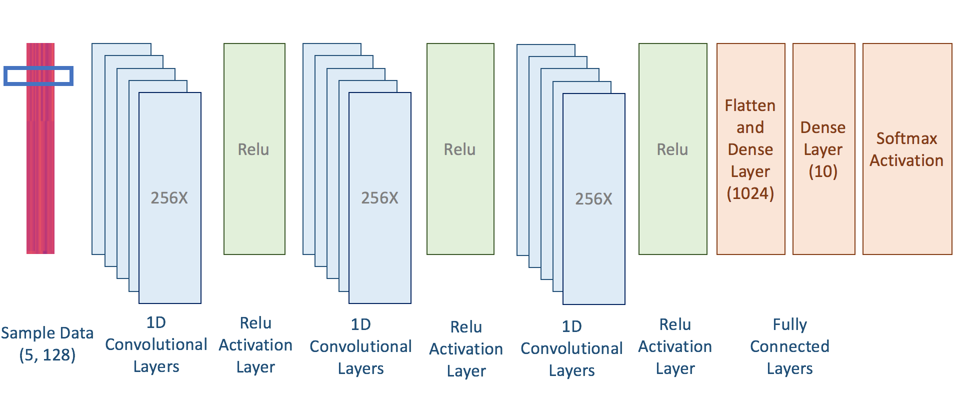
If you look closely at the final architecture, you will notice that I did not use either dropout or Pooling. The reason for this is that the shape of each of the sample is (5, 128), so it does not makes sense to pool across a vector of length 5. Similarly, because of the shape the number of neurons at each of the layer will only be 5, so dropping half of them might not give the best results. However, I did use dropout before by last layer (you can check this in the code) as there I have plenty of neurons (1024 to be exact). Finally, I trained my model for 10 epochs with early stopping, i.e. if my validation accuracy did not increase for certain number of epochs then I stop training it further. I initially tried training for 25 ecpochs but I never saw improvement after 7-8th epoch. The model achieved an accuracy of 62% on the validation set, which is a far cry from the benchmark of 84% , but is still a lot better than a random guess of 10%.

If you have any questions please leave a comment!

Cheers!!